Implicit Factor Model - A Cross-Sectional Regression Approach

 

Equity Factor Models - Build one in R with a few lines of codes

A step-by-step guide to build your own fundamental factor model using R and cross-sectional regressions

Alexander Popov — unsplash

Multi-factor models are a must-have for investors looking to understand their portfolio’s performance drivers. It helps explain the actual return of factors such as countries, sectors, and styles, independent of other factors’ effects.

In this article, we will focus on the mechanics of such models, and how to code them in R. We also introduce a visualization that lets you visualize the factor performance contributions overtime.

A Factor Model, what’s that?

A factor model also called a multi-factor model, is a model that employs multiple factors to explain individual securities or a portfolio of securities.

It exists at least three types of factor models:

• Statistical factor models — They use methods similar to principal component analysis (PCA). In these models, both factor returns and factor exposures are determined from asset returns. Factors are “statistical” in the sense that they cannot be interpreted. They bear names such as “loading1”.
• Explicit factor models — These models use techniques such as time series regression to determine factor exposures. They take in input asset returns as well as factor returns. For example, these are the models you use to assess macro indicators’ impact on a portfolio. Disadvantages are that they sometimes produce counterintuitive exposures and tend to have low predictive power.
• Implicit factor models — These models require returns and factor exposure for each security. The output is the implied return of each factor. They use techniques such as cross-sectional regressions. These models are easy to interpret and provide clear, actionable insights. However, they are data-intensive and require the factor exposures of all securities.

We will focus on implicit factor models and their implementation in R.

The math behind factor models

Implicit factor models are estimated by running a cross-sectional regression. A cross-sectional regression is a type of regression that looked at variables at a single point in time.

Cross-sectional regression formula takes the following form:

Formula of cross-sectional regression — Image by Author

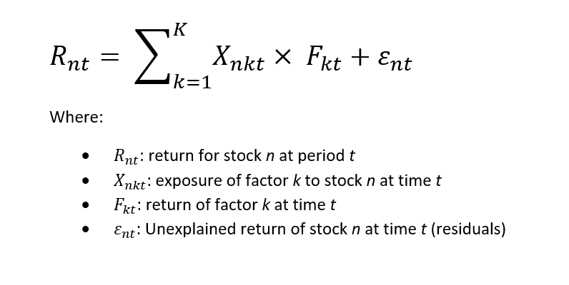
This formula takes stock’s returns and their exposures to factors as input for each stock. The output after fitting is the return for each factor that minimizes the epsilon in the formula.

A global universe of 3000 stocks and a factor model with 100 factors such as market, countries, sectors, and styles will produce the following system of equations to fit:

Cross-sectional formulas to fit. 3000 stocks, 100 factors for 30'000 input params — Image by Author

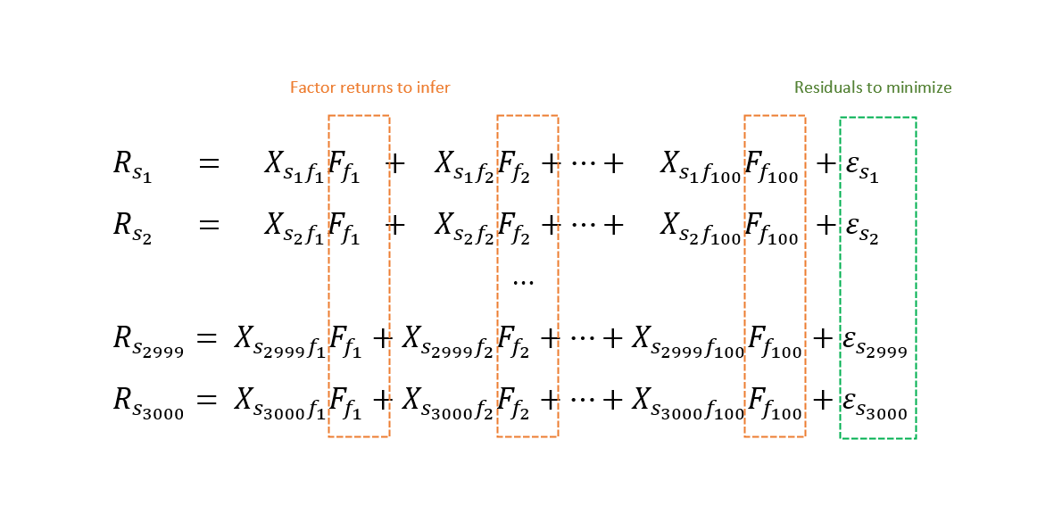
Note that the only common variables among these equations are the factors implicit return that we want to find. When fitting this system, we have to specify that we want these to be constant among the equations.

Our goal is to find F1 to F100 to minimize the sum of the epsilons (residuals). In other terms, to find the implicit factors returns that explain most of the return of stocks.

Factor definitions and exposures — Dummy and Z-scores

Most of the multi-factor models use the following factors to explain stock’s returns:

• Market intercept: Represents the fact that all stocks are part of the stock market. It always takes the value of 1 and can be interpreted as the intercept of the regression.
• Country factors: Exposure to these factors takes the form of a dummy variable, 1 if a stock belongs to the country and 0 otherwise. Country factors are only for multi-countries models.
• Sector factors: Like country factors, they take the form of a dummy variable, 1 if a stock is in a sector and 0 for the other sector factors.
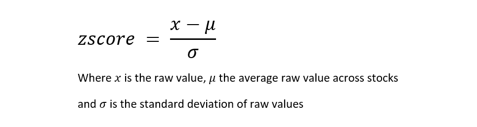
• Styles factors: These are factors such as Value, Momentum, Low Risk, Quality, and Size. Factor’s exposures are defined in terms of z-scores. A z-score is a measure of how far from the mean a data point is. It is used to normalize raw data and is expressed as the number of standard deviation below or above the average value.

Z-score formula — Image by Author

We use generally accepted definitions for our style factors. These have to be chosen carefully to avoid collinearity. Something to keep in mind.

Regression weights

Not all equations of the cross-sectional regression should have the same weights. Intuitively, larger stocks should have more influence as they are most likely driving the market. However, we do not want to use an approach such as market cap weighting that would put too much emphasis on larger market cap stocks.

A good compromise is to use the square root of the market cap as a weighting scheme for our equations. According to Bloomberg’s white paper, this is what is used by their equity model in their <PORT> function.

Formula to get the weight of each equation in our regression — Image by Author

Normalization of Style factors with z-scores

Z-scores are highly sensitive to the distribution of the underlying data. For example, the size factor, often measured by the market cap of stocks, is usually skewed toward smaller market cap stocks. A vast majority of stocks are below a few billion dollars market cap while few can reach above 100 billion and even trillions like Apple or Amazon.

Market Cap & Z-score distributions (capped at +/-3). Z-scores average is heavily skewed toward 3 - Image by Author

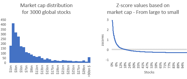
This kind of z-score distribution is not ideal. The average is skewed toward 3, and this will impact our calculation and the implicit return computed. For this reason, we need to modify the distribution, so it becomes a standard normal distribution. It is done by computing z-scores of z-scores until our z-scores have a market-cap-weighted mean of 0 and a standard deviation of 1.

There is another benefit of doing this; A market portfolio, a theoretical portfolio made up of all the stocks available in our investment universe, need to be logically explained by the market factor (it is called “market” portfolio after all). With our modified z-score distributions, all style factors have a 0 exposure, leaving only the market factor explaining the market portfolio performance (ignoring country and sector factors which will be taken care of by our regression constraints)

Market portfolio is only exposed to the market factor after our style’s z-score normalization (ignoring country and sector factors) — Image by Author

Finally, we need to limit extreme values by clipping z-scores between 3 and -3.

Regression constraint

Additional constraints need to be imposed on the cross-sectional regression to avoid collinearity among factors. Country factor exposures suffer from collinearity with the market factor. It means that a linear combination of country factor exposures can reproduce the market factor exposure. The same applies to Sector factor exposures.

Besides, a market portfolio should only be explained by the market factor (intercept). It makes little sense to have the market portfolio explained by factors other than the market factor.

Therefore we need to add a matrix of restrictions to our regression. This matrix imposes that the country factor returns (or sector) sum to 0 at the market level. This way, we force our regression to ensure that the market portfolio is only driven by the market factor and avoid any collinearity issue from country and sector factors.

Market portfolio is only exposed to the market factor thanks to our restrictions (ignoring style factors) — Image by Author

Our restrictions matrix (M) consists of the weights of each factor in our market portfolio. Our constrained regression will solve implicit returns of factors such as their weighted sum (as given by our restriction matrix) equals 0.

Our restrictions matrix M multiplied by a vector Beta of estimated factor returns such that it produces a vector of zeros — Image by Author

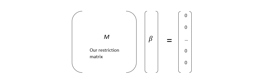
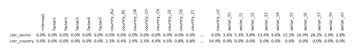
The result is a matrix with one row for the sector constraint and another row for the country constraint. Weights for each factor match the factor exposure in the market portfolio.

Example of restrictions matrix. Sum of each row equals to 100% — Image by Author

Data preparation and stocks z-scores

To fit our cross-sectional regression, we need to feed our model with data. For this article’s sake, we skip the details of the creation of these data and focus only on the format.

Our code will take in input two files:

• Data file: List of stocks with all their factor exposures. One stock per row and one factor per column. Also, we have the total return column and the weight column (square root of market cap weighting).
• Restrictions matrix: List of restrictions on our model with two rows corresponding to the country and sector restrictions.

These files are available on the following GitHub repo.

Build your own Custom Factor Model in R

Time to build our custom model using R. The full code is available in this GitHub repo.

This code is a wrapper to the function systemfit from the R package ‘systemfit’. Systemfit is ideal for performing a cross-sectional regression with restrictions. However, one of the drawbacks is that it cannot allow Seemingly Unrelated Regressions (SUR) models with equation-specific weights. Explanation of SUR is out of the scope of this article but more information can be found on wikipedia.

Load the data

First things first, we need to load our data files into variables. Make sure your R working directory contains our two files.

#################################################################
#  LOAD THE DATA
#################################################################
# EXPOSURE DATA
data_filename = "data.csv"
factor_data <- data.frame(read.csv(data_filename))
# MATRIX DATA
constraints_matrix_filename = "constraints_matrix.csv" 
constraints_matrix <- data.frame(read.csv(constraints_matrix_filename))
constraints_matrix <-  as.matrix(constraints_matrix[ ,!(colnames(constraints_matrix) %in% c("X"))])

Prepare the data for the regression

The next step is to modify the data from our data file to ensure that style’s z-scores have a mean of 0 and a standard deviation of 1 and reflect the different equations weighting.

The below code transforms our z-score distributions to ensure they have a weighted mean of 0 and a standard deviation of 1.

#################################################################
#  FORMAT THE ZSCORES TO CREATE STANDARD NORMAL ZSCORES
#################################################################
list_factors <- c('factor1','factor2','factor3','factor4','factor5')
for (istyle in list_factors) {
  print(istyle)
  zscores_values<- factor_data[,istyle]
  zscores_new_values<- factor_data[,istyle]
  ZscoresSum<- 0
  print(abs(weighted.mean(zscores_values, factor_data$wgt, na.rm=TRUE)))
  # ITERATE ZSCORE CALCULATION UNTIL THE ZSCORE DISTRIBUTION HAS A WEIGHTED MEAN OF 0 AND A STDEV OF 1
  while ( (abs(weighted.mean(zscores_values, factor_data$wgt ,na.rm=TRUE)) > 0.0001 | abs(sd(zscores_values,na.rm=TRUE)-1) > 0.0001 ) & ZscoresSum != abs(weighted.mean(zscores_values, factor_data$wgt,na.rm=TRUE))) {
    ZscoresSum <- abs(weighted.mean(zscores_values, factor_data$wgt,na.rm=TRUE))
    zscores_new_values <- zscoreweighted(zscores_values, factor_data$wgt, 3, -3)
    
    if (abs(weighted.mean(zscores_new_values, factor_data$wgt ,na.rm=TRUE) ) < abs(weighted.mean(zscores_values, factor_data$wgt, na.rm=TRUE))) {
      zscores_values = zscores_new_values
    }
    print(abs(weighted.mean(zscores_values, factor_data$wgt ,na.rm=TRUE)))
  }
  
  factor_data[,istyle] <- zscores_values
}

Unfortunately the package ‘systemfit’ cannot estimate Seemingly Unrelated Regressions (SUR) models with different weights on equations. To go around this limitation we will repeat the rows of our dataset by their weight multiplied by 100'000. It is not perfect but it does the job.

Example of rows repeated to overweight them in the regression — Image by Author

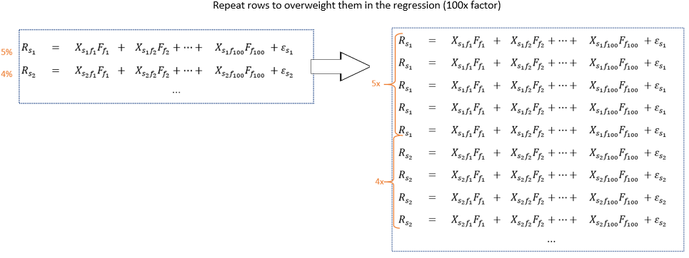
And here is the R code to do it.

factor_data$wgt = round(factor_data$wgt * 100000)
factor_data_for_fit = expandRows(factor_data, "wgt") # Column wgt contains square root of market cap weights

Run the regression

We now apply the systemfit function to perform our regression. This function takes for input the formula, our data, and our restrictions matrix.

The following line of code generates our regression’s formula:

#################################################################
# BUILD FORMULA
#################################################################
formulaSectorStyleRegression <- as.formula(paste("total_return_1d ~ 1 + ", paste(colnames(factor_data[ ,!(colnames(factor_data) %in% c("X","Intercept", "total_return_1d", "wgt"))]), collapse= "+")))## OUTPUT
# total_return_1d ~ 1 + factor1 + ... + sector_59 + sector_60

And finally we execute the line below to run our regression.

#################################################################
#  PERFORM CROSS SECTIONAL REGRESSION WITH SYSTEMFIT (SUR:  Seemingly Unrelated Regressions)
#################################################################
CrossSectionalFit <- systemfit(formulaSectorStyleRegression, "SUR", data=factor_data_for_fit, restrict.matrix=constraints_matrix, 
                               pooled = TRUE, methodResidCov ="noDfCor", residCovWeighted = TRUE )

We used the parameter “pooled = TRUE” to restrict coefficients to be equal in all equations, and “method = “SUR” to use the estimation method “Seemingly Unrelated Regressions”.

Get the regression statistics and coefficients

Use the following code to extract the regression’s output, such as R2 and variable coefficients.

#################################################################
#  REGRESSION RESULT
#################################################################
CrossSectionalFitAtDate <- coef(summary( CrossSectionalFit ))

Code to extract factor loadings:

#################################################################
#  FACTOR IMPLICIT RETURN AND FACTOR STATS
#################################################################
FactorModelResults <- data.frame(factornames)
i_factor<- 1
for(i_factor in 1:length(factornames)){
  
  if (factornames[i_factor]=="Intercept") {
     FactorModelResults[i_factor,"FactorReturn"] <- CrossSectionalFitAtDate ["eq1_(Intercept)", "Estimate"] 
     FactorModelResults[i_factor,"TStat"] <- CrossSectionalFitAtDate ["eq1_(Intercept)", "t value"] 
     FactorModelResults[i_factor,"PValue"] <- CrossSectionalFitAtDate ["eq1_(Intercept)", "Pr(>|t|)"] 
     FactorModelResults[i_factor,"Standard Error"] <- CrossSectionalFitAtDate ["eq1_(Intercept)", "Std. Error"]
  } else {
     FactorModelResults[i_factor,"FactorReturn"] <- CrossSectionalFitAtDate [paste("eq1","_", factornames[i_factor],sep=""), "Estimate"] 
     FactorModelResults[i_factor,"TStat"] <- CrossSectionalFitAtDate [paste("eq1","_", factornames[i_factor],sep=""), "t value"] 
     FactorModelResults[i_factor,"PValue"] <- CrossSectionalFitAtDate [paste("eq1","_", factornames[i_factor],sep=""), "Pr(>|t|)"] 
     FactorModelResults[i_factor,"Standard Error"] <- CrossSectionalFitAtDate [paste("eq1","_", factornames[i_factor],sep=""), "Std. Error"]
  }
  
}

Code to extract the model statistics:

#################################################################
#  R-SQUARED OF MODEL
#################################################################
RsqData <- data.frame(c(summary( CrossSectionalFit$eq[[1]])$r.squared),c(summary( CrossSectionalFit$eq[[1]])$adj.r.squared),c(summary( CrossSectionalFit$eq[[1]])$sigma))
colnames(RsqData) <- c("R2","AdjR2","EstimatedStandardErrorOfResiduals")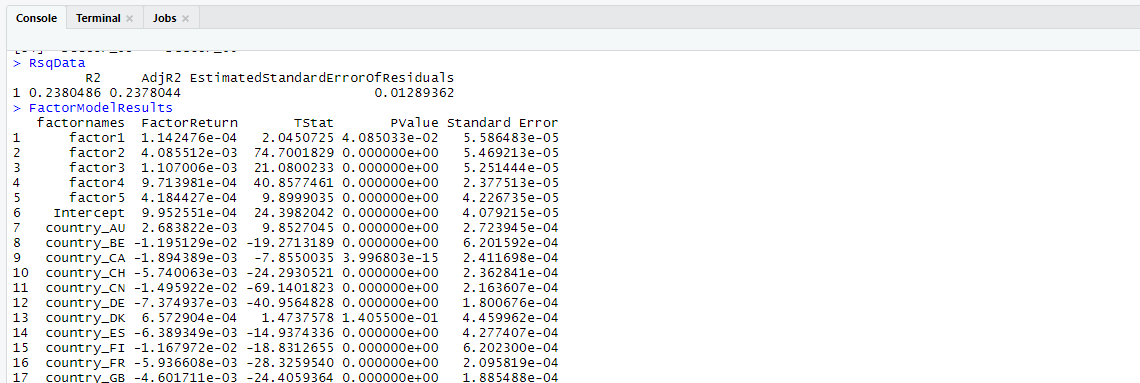

Rstudio screenshot showing the result of the cross-sectional regression — Image by Author

Output and visualization — Example of Amazon performance breakdown

Thanks to the R code presented, we can compute implicit factor returns for one date. Repeating the process for additional dates will produce time series for factors. Each factor is net of other effects, and individual factor’s contributions sum up to the total performance of a stock or portfolio.

Below is an example of performance breakdown visualization for Amazon. This chart shows the November 9th market reversal following the covid-19 vaccine news and its impact on Amazon (harmful residuals and reduction of the momentum factor positive contribution). Note that factors contribution on each day sum up to Amazon’s stock return.

Example of visualization to analyze the performance drivers of a stock — Image by Author

A word of caution regarding our code and methods; we presented a basic factor model that ignores many details of advanced models, such as handling missing factors and stocks different market open hours.

Conclusion

In this article, we demonstrated that a multi-factor model can be coded in a few lines of R.

Custom factor risk models are a must-have for any investors looking to understand their portfolio’s performance drivers. It helps validate the actual return of factors, net of other effects, and lead to better insights for your portfolio management and stocks selection. I recommend anyone investing in the stock market to take a look at them. I believe they are no longer reserved for sophisticated investors and would, without any doubt, benefit retail investors.

The next step in building your custom model is to pick your factors. There are many ways to do it, and I am preparing another article on the most common choices to select your style’s factors.

Reference

• Sample data & R code, https://github.com/charlesmalafosse/custom-factor-model.
• Arne Henningsen and Jeff D. Hamann (2007). systemfit: A Package for Estimating Systems of Simultaneous Equations in R. Journal of Statistical Software 23(4), 1–40. http://www.jstatsoft.org/v23/i04/.
• Ercument Cahan and Lei Ji (2016), Global Equity Fundamental Factor Model, Bloomberg Whitepaper.
• Seemingly Unrelated Regressions (SUR), Wikipedia, https://en.wikipedia.org/wiki/Seemingly_unrelated_regressions
• Enhancing the Investment Process with a Custom Risk Model, Axioma Case Study, September 26, 2013.